(Watch the “Spreadsheet Basics for Journalists, Part 1” video to see a demonstration of the techniques covered on this page)

First: Make a plan.

Smart journalists prepare for an interview by thinking up good questions to ask. Do the same thing before you begin a data analysis. The audiences journalists write for are most interested in information that exhibits impact, timeliness, prominence, proximity, novelty, conflict, and/or currency. So you might want to try to learn, for example, whether anyone’s raise was unusually large or small compared to the average, and what the total impact of the raises will be on the city’s finances.

To help you learn both of those things, Google Sheets will need each department head’s name, old salary and new salary, arranged so that each department head’s information appears in its own horizontal row, and each type of information (name, old salary, new salary) appears in its own vertical column. Fortunately, the mayor’s table matches that arrangement exactly, so let’s try opening a Google Sheet, then simply copying-and-pasting the data from the mayor’s table into it. Then, we’ll use do a quick calculation of each department head’s raise. I’ll describe each step below, with pictures and videos to help you see what to do.

Logging into Google Drive and creating a Google Sheet

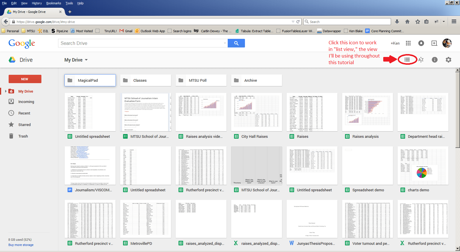
Getting into Google Drive. Click on drive.google.com, using whatever Web browser you’re using to view this page. I’m using Firefox on a PC, but using Safari on a Mac or any other combination of browser and computer type should work just fine. You should see a page that looks something like this:

If you have a Google account (for example, a Google Gmail account), go ahead and sign as you usually would. If you don’t, click “Create an account” and follow the instructions to set up a Google account. It’s free, and it’s a truly handy thing to have.

Once you’ve signed in, your screen should look like one of the two pictures below. The first picture shows Google Drive’s “Grid View,” and the second shows Google Drive’s “List view.” You can use whichever view you prefer, but I’ll be using the “List view,” so if you want to use “List view” as well, just click the icon I’ve circled in the “Grid view” picture.

I use Google Drive a lot, so I have all kinds of files already. Yours may have fewer files, or it may be empty.

“Grid view”

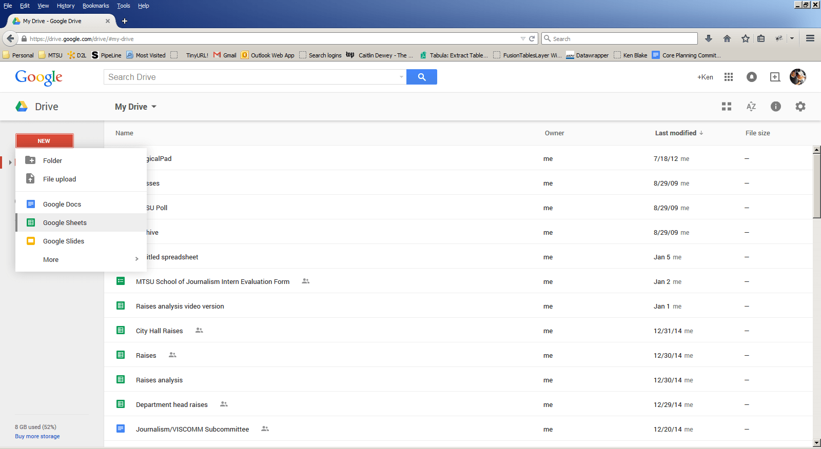
“List view” (the one I’ll be using):

Creating a blank Google Sheet. Now, make a new Google Sheet by clicking “New” in the red box in the upper-left corner of the page, then clicking “Google Sheets” on the menu that opens. Like this:

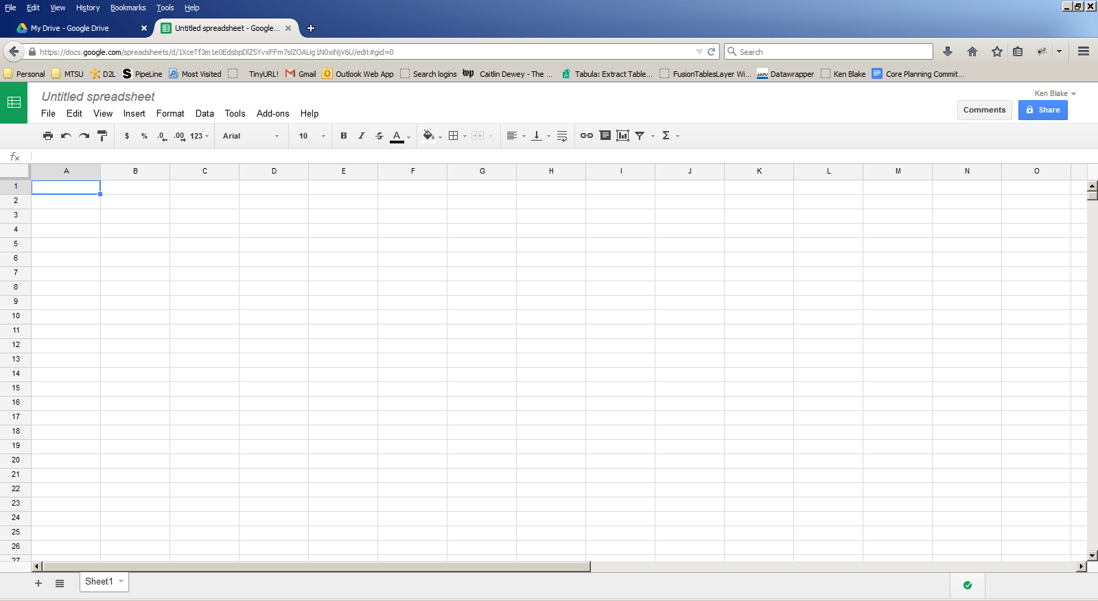
A blank Google Sheet should open in a new window. Like this:

Copying and pasting the salary data into your blank Google Sheet. Now to get the salary data into this blank Google Sheet so you can do something with it. There are lots of ways to get data into a Google sheet. You could, for example, simply type it in. But that’s a lot of work, and you’ll probably make a few mistakes. If you already have the data in a file on your computer, you could try importing it by clicking “File / Import / Upload,” then browsing to the file on your computer. You can fiddle with those approaches later, if you like. For this example, we’re going to simply copy and paste it from the table you saw back on the “Spreadsheet Basics” web page. Go back there, left click on the table’s “Name” column heading and, holding down the left mouse button, drag until you have highlighted all of the salary information, including the last figure: 56185. Then, release the mouse button, hold down the “Ctrl” key on your PC keyboard (or the “Command” key on your Mac keyboard), and press the “c” key to copy the data you’ve highlighted.

Then switch back to the Google Sheet window, click on the first box in the spreadsheet’s upper left corner, and hold down the “Ctrl” key while pressing “v” or, if you’re using a Mac, hold down the “Command” key while pressing “v.” Doing so should paste the salary data into the Google Sheet, like this:

You might notice that the “Name” column isn’t quite wide enough to show some of the names in their entirety. To automatically widen the column enough to show the whole of each name, move your mouse pointer to the dividing line between the “A” and “B” labels at the top of the “Name” and “Old salary” columns until you find the spot at which your mouse pointer changes to a double-ended arrow. Then, just double click. The column will widen automatically. If you have trouble with this part, watch for it in the video. It’s not an easy thing to get a screen shot of.

Calculating Daniel Anderson’s raise. This part might be a little unimpressive. It might look like a lot of work compared to just pulling out a pocket calculator. But hang on; if you’ve never seen a spreadsheet in action, you’ll soon see that a spreadsheet can run circles around a calculator. So, stick with me, OK?

To figure the size of Daniel Anderson’s raise, we need to subtract his old salary, 49190, from his new salary, 54109. On your calculator, you would punch in 54109, hit the minus key, punch in 49190, then hit the equal key, and the calculator would show that Anderson’s raise is 4919, or $4,919. You’ve probably known how to do that since grade school.

To understand how a spreadsheet approaches the same problem, you’ll have to hearken back to something else you probably learned in grade school: plotting points on a grid. The teacher would give you a paper grid and pair of “coordinates,” and you had to pencil in a dot on the grid at the position the coordinates indicated. I’m happy to tell you that the payday for learning that skill has finally arrived. You see, your new Google Sheet is smart enough to know that when you pasted the salary data into it, Anderson’s new salary landed at the intersection of Column C and Row 2, a box, or cell, that your Google Sheet understands to be “Cell C2”:

To tell your Google Sheet to find Anderson’s raise, all you have to do is tell it to take the number in cell C2 (Anderson’s new salary) and subtract from it the number in cell B2 (Anderson’s old salary). To do so, click on a handy blank cell – let’s use cell D2 – type an equal sign, click on cell c2, type a minus sign, click on cell B2, and press “Enter.”

While you are typing these instructions, your screen should look like this:

After you’ve hit “Enter,” click on cell D2, and you should see this:

This little exercise has revealed one advantage a spreadsheet has over a calculator: Once you’ve gotten a number into a spreadsheet, you never have to type it again. Any time you want to do something with it, all you have to do is point to its location. That’s faster, and it eliminates the possibility of typos.

But there’s more. Here comes the impressive part I promised a moment ago.

See that little blue square in the lower right corner of cell D2? Click on it with your mouse (when you’re on exactly the right spot to click, you mouse pointer will change to a large “plus sign” shape), hold down the left mouse button to “grab” the square, drag down to cell D23, just to the right of Thomas Wilson’s new salary of 56815, then release the left mouse button. If you did all of that correctly, your Google Sheet will instantaneously calculate the raise for each of the other 21 department heads, from Michael Brown down to Wilson. The results should look like this:

Try that with a calculator! A spreadsheet’s ability to work based on each value’s location, rather than just the value itself, gives the spreadsheet tremendous speed and flexibility. Also, if you ever change a value in a spreadsheet, any calculations that value is involved in will automatically recalculate. For example, try changing Anderson’s new salary to 55000 by typing 55000 in place of the original 54109 and then pressing “Enter.” The instant you hit “Enter,” the amount of his raise will update to 5810, which is 55000, Anderson’s original salary of 49190.

To finish up, add a bold-faced “Raises” heading to cell D2 so we can keep track of what the column shows. Also, don’t forget to change Anderson’s new salary back to 54109.

Recap

In this part, you’ve learned how to log into Google Drive, create a Google Sheet, copy and paste data into the sheet, automatically resize a column, identify a cell’s location based on its column (vertical) and row (horizontal) position, program a simple calculation, and copy that calculation into other cells.

Go to Part 2: Describing and Comparing the raises

Go to Part 3: Making an interactive graphic